Single-Mode Connector Attenuation Estimation
In the latest installment of our “Connector Basics” series, Randy Manning of APEX explains basic single-mode connector attenuation estimation using Monte Carlo simulation.
 An optical fiber connector is a mechanical component that transfers light between two fibers or between a fiber and an active device such as a transmitter or receiver. A connector is intended to easily mate and un-mate repeatedly over its service lifetime. A permanent or semi-permanent connection between two fibers is called a splice.
Electrical connectors and fiber-optic connectors both perform the same function, transmitting a signal between two components and mechanically interconnecting them. In the case of an electrical connector interconnecting two wires, the electrical signal, in the form of electrons, is transmitted through both the wires and the connector itself. However, in the case of an optical connector interconnecting two fibers, the optical signal, in the form of photons, is transmitted only through the optical fibers and not the actual connector, with the exception of an optical connector containing an optical element such as a lens. An optical connector is, therefore, only a mechanical device, whereas an electrical connector is an electromechanical device.
Electrons can follow a rather winding path through electrical conductors and connectors without significant losses, so long as sufficiently good electrical contact is made at all permanent and separable interfaces. Electrical connectors require a relatively low level of precision to effectively transmit a signal. Photons, on the other hand, travel in a straight line and when unconfined, radiate and spread, reducing optical signal intensity and loss when not precisely aligned at connector and splice interfaces.
Due to the small size of the mode fields (or cores) in optical fibers, a relatively high level of alignment precision is required between fiber ends to transmit an optical signal across permanent and separable interfaces without significant losses. Optical fiber connectors, therefore, require a very high degree of mechanical precision to minimize losses between two mated fibers. Typical tolerances of size and location for electrical connector component features are about 0.1mm, whereas typical tolerances of optical fiber connector component features, which align the fibers, are about 0.001mm (1 micrometer).
The primary measure of the quality of the transmitted signal in an optical fiber connector is called attenuation, the portion of the signal lost across the separable interface. Lower attenuation is better for optical components such as connectors or splices. Attenuation is sometimes referred to as insertion loss. Attenuation is typically defined as a percentage of power lost or in the logarithmic form as decibels, both forms being dimensionless.
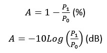
When the logarithmic form is used, it becomes a simple matter of adding the attenuation of various components together to determine the overall loss of a fiber link. It should also be noted that the negative sign in the decibel form is a matter of convention and it may be absent in some presentations, in which case the attenuation is given as a negative value, i.e. -1.0dB instead of 1.0dB.
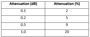
The following table provides the equivalent attenuation in decibels and percentage power lost.
Attenuation or loss is measured between two mated pair of fiber-optic connectors, which consist of two plugs that contain optical fibers and a mating adapter and usually a sleeve to align the two connector plugs. These are arranged in a plug-adapter-plug configuration. A typical optical fiber plug contains an alignment portion known as a ferrule. Commonly, the ferrule is a cylindrical component with a precision fiber bore located in the center of the outside diameter. An optical fiber is fixed in the precision bore with an adhesive. Ideally, the fiber is polished flush with the ferrule end face, which usually is spherical.
Let’s consider single-mode fibers in our connector attenuation example. Connector attenuation or loss mechanisms are comprised of a number of misalignments or offsets between mated connector fiber pairs. These misalignments include:
- Lateral offset between the mated fiber axes
- Angular offset between the mated fiber axes
- Longitudinal offset (separation) between the mated fiber end faces
Additional connector loss mechanisms include:
- Mode-field diameter mismatch between mated fibers
- Reflections at the fiber end faces due to index of refraction differences
Modern low-loss optical fiber connectors eliminate longitudinal offset losses and reduce reflection losses by placing the fiber ends into physical contact. Physical contact (PC) reduces the end face reflections by eliminating the air gap between the fiber ends. A portion of the light is reflected whenever it encounters an index of refraction difference between two different materials such as glass and air.
When the fiber end faces are assumed to be in physical contact, the following loss mechanisms must be considered.
Lateral Offset
Fiber and ferrule feature tolerances that contributed to lateral offset include:
- Fiber core-to-cladding concentricity tolerance
- Fiber cladding diameter
- Ferrule fiber bore diameter
- Ferrule bore to ferrule outside diameter concentricity tolerance
- Ferrule diameter
- Alignment sleeve diameter
Angular Offset
Fiber and ferrule tolerances that contribute to angular offset include:
- Fiber bore to ferrule outside diameter angle tolerance
- Fiber cladding diameter to ferrule fiber bore diameter clearance angle tolerance
- Ferrule diameter to alignment sleeve diameter clearance angle tolerance
Mode Field Diameter Mismatch
Fiber tolerances that contribute to mode-field diameter mismatch include:
- Nominal fiber mode field diameters
- Fiber mode field diameter tolerances
Fiber and Ferrule Tolerances
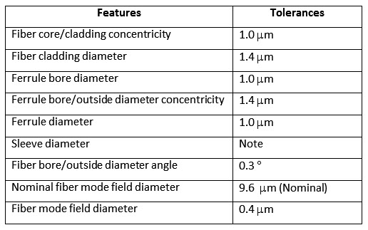
[Note: Resilient sleeve diameter tolerance is included in ferrule diameter tolerance.]
Probability Density Distribution
The primary loss mechanism in a typical optical fiber connector is lateral offset. While angular offset and mode-field diameter mismatch loss also add to the loss between two connector pair, they are usually small in comparison to the lateral offset loss.
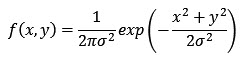
It is assumed that the ferrule and fiber dimensional tolerances that contribute to lateral offset are normally distributed in Gaussian distributions. The position of the fiber-core center relative to the ferrule center can be described as having a substantially bivariate normal distribution. The bivariate probability density function is given as:
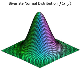
The bivariate normal distribution is shown in the following figure.
The fiber and ferrule tolerances that contribute to the lateral offset of the fiber core center relative to the ferrule center can be combined statistically to determine the value of the standard deviation σ of the probability density function. This combination yields a value for σ of approximately 0.4μm in our example. Because the bivariate distribution function is the joint probability of two independent normal distributions, we can use Monte Carlo simulation methods to generate random values for the x and y offset of the fiber cores from the ferrule center for a given number of connectors. A scatter plot may then be made of the x and y offsets as shown in the following figure.
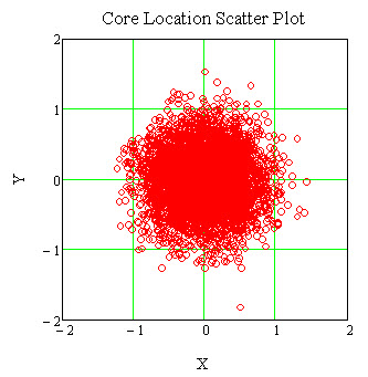
This figure is a Monte Carlo simulated two-dimensional representation of the preceding three-dimensional bivariate normal distribution graph.
A set of random values for the x and y offset of the fiber cores from the ferrule center may be generated that correspond to a second set of connectors. A scatter plot representing the x and y offsets of mated connector pair may be made, the figure of which follows.
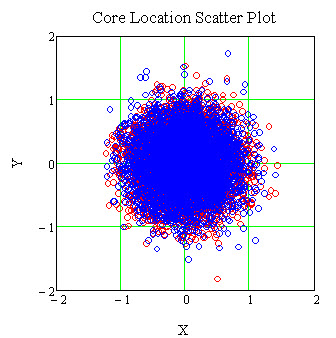
Lateral Offset
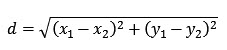
Each core location for the two connector sets is shown in a different color. The distance between any two randomly selected core centers for the different connector sets determines the lateral offset between the two randomly mated connector pair. The distance between two selected core centers is given by the distance formula:
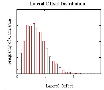
The lateral offset of all the connector pair in the set may now be determined and a histogram constructed to show the distribution of the random mated connector pair offsets. The mean value of the lateral offset is 0.71μm and the standard deviation is 0.37μm. The histogram is shown in the following figure.
Connector Attenuation
Once the lateral offset of the mated connectors is known, the mated-pair connector attenuation may be determined for the connectors. The mode field radius is 4.8μm, corresponding to a nominal 9.6μm mode-field diameter.
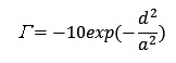
Where: Γ = attenuation (dB)
d = lateral offset of fiber cores (μm)
a = mode-field radius (μm)
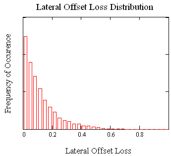
The mean value of the mated-pair connector attenuation is 0.12dB and the standard deviation is 0.12dB. A histogram showing the mated-pair connector attenuation or loss distribution corresponding to the core offsets described in the previous figure is shown as follows.
The loss due to angular offset and mode-field diameter mismatch can be simulated in a similar fashion and combined to determine the total connector attenuation. Additionally, the probability that a certain percentage of the mated connector pair population will have attenuation values less than a given value can also be determined from Monte Carlo simulation.
Monte Carlo simulation is a useful tool for analyzing optical, electrical, and mechanical components to estimate the field performance and manufacturability of a product. It is a capability to which all connector designers, manufacturers, and users should have access.
Visit APEX Electrical Interconnection Consultants online.
[hr]
 Randy Manning is a senior consultant at APEX Electrical Interconnection Consultants. He has 44 years experience in interconnection technology in fiber optic and electrical interconnection products and has developed many types of interconnection products including fiber optic connectors and optical fiber splices and optical device packages. As a private practice consultant, Manning has been involved in fiber optic interconnection and electrical connector technology development and standardization. Previously, he was a development manager and principal engineer at Tyco Electronics and AMP Incorporated.