Replacing Printed Wiring with Engineered Cable Solutions for High-Speed Applications
Getting faster transmission through interconnects is not as simple as just turning up the speed with a dial. It requires adjustments to signal modulation and SerDes technology, as well as advancements in interconnectivity and IC packaging.

Since networking equipment operating at 100G, 200G, and 400G total data rate per port has become ubiquitous, network system development engineers have shifted their focus to 800G port data rates and the new 1.6T per port. However, getting faster transmission through interconnects is not as simple as just turning up the speed with a dial. It requires adjustments to signal modulation and SerDes technology, as well as advancements in interconnectivity and IC packaging. Figure 1 relates data rate to the required bandwidth in gigahertz and illustrates some of the changes.
Assuming an OSFP IO solution, a data rate of 200G uses NRZ modulation — a two-level modulation. As the data rate increases from 200G to 400G, the channel frequency requirement stays almost the same. Instead of increasing bandwidth, the data rate is doubled by changing the modulation to PAM4 — a four-level modulation. Simply put, for every one bit sent with NRZ, two bits are sent through the channel with PAM4. As data rates increase to 800G, PAM4 remains, and the frequency required doubles. Other modulations may be in the works for data rates beyond 1.6T.
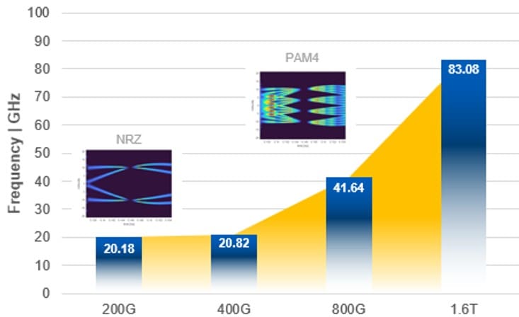
Figure 1 | OSFP data rate vs. 99.9% frequency content. Modulation is shown near relevant data rates.
Changing the modulation and increasing the bandwidth does introduce some engineering challenges. When the modulation changes from NRZ to PAM4, the available signal magnitude (also known as eye height, named for the opening that looks like an eye, observable in the NRZ and PAM4 diagrams in Figure 1) is decreased by 33%. Lowering the signal magnitude means the signal-to-noise ratio is immediately affected, making PAM4 signals more susceptible to noise. When bandwidth increases, two transmission parameters are affected: rise time and insertion loss. Rise time is the speed a voltage transitions from one level to another. With faster rising edges, reflections in the channel become stronger and noisier. Simultaneously, higher frequencies have higher insertion loss, and more insertion loss means less signal. In summary, for 800G and 1.6T data rates with OSFP, the modulation lowers the available signal magnitude, there is more noise from higher reflections, and there is less signal from higher insertion loss.
Interconnect manufacturers provide solutions to overcome these problems, such as the use of products designed to bypass PCB traces with twinaxial cable. Figure 2 displays typical applications for the cabled transmission line product families.
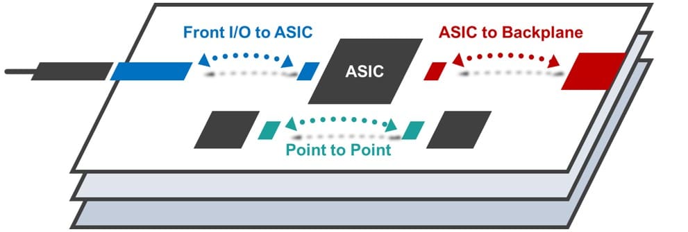
Figure 2 | Cable transmission line applications
Figure 3 and Figure 4 show how these solutions improve insertion loss performance. Insertion loss is reported in decibels (db), and anything above 0 is gain. Since interconnects are passive devices, all insertion loss is less than 0 db. The lower the number for the insertion loss, the less signal is available. For this reason, insertion loss is sometimes reported as a positive number to make the name match the chart. However, it is standard practice to report insertion loss as a negative number.
To show how cable can improve insertion loss, two metrics are presented: the loss reduction multiplier of using cable and the insertion loss of the cable over frequency. At 200G and 400G data rates, transmission line lengths can be about four times as long by using cable, and at the 1.6T data rate the length reaches can be over six times as long. For 200G and 400G, the length of the transmission line could be achieved with PCB alone. So even though there was an advantage to using cable, there wasn’t a need. Now at 800G and 1.6T data rates, the signal loss is so high that the system will not work with only a PCB and, at these speeds, the advantage aligns with the need.
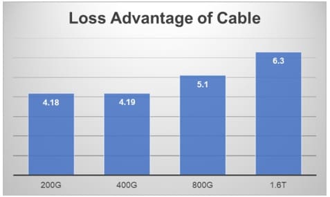
Figure 3 | Relative change between cable insertion loss and PCB insertion loss

Figure 4 | Cable insertion loss and PCB insertion loss
By carefully designing the interconnects, reflections can be mitigated. As an example, the reflection parameters, impedance, and return loss of the 800G OSFP are presented in Figure 5.
Impedance is a plot of reflections in time, and these reflections are measured in ohms. The entire mated OSFP connector system changes in impedance by only six ohms. As a frame of reference, production printed circuit boards for this application are controlled within +/- 7.5 ohms, making the OSFP well below the expected impedance changes in the system.
Return loss is a measure of the reflections in the frequency domain. For reference, the return loss for RF connectors should be below -20 db in the working frequency-band. For the required signal integrity performance, the return loss should be as low as possible and below -12 db at the Nyquist frequency (the frequency that is one half the data rate for NRZ and one quarter the data rate for PAM4) for the application. In this case, the Nyquist frequency is 26.56 GHz, and the return loss at that frequency is clearly under -12 db. In summary, the reflections are low and well controlled within the 800G application frequency band, which operates at 112 Gb/s signaling speed per channel.
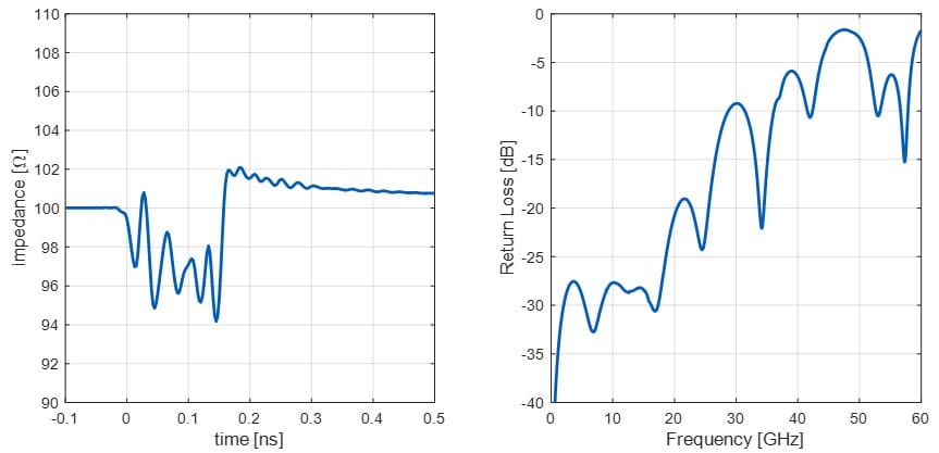
Figure 5 | 112G OSFP impedance and return loss
Many cabled products, with this level of performance, are available today. There have been many demonstrations of the increasing performance levels of these products at multiple industry events, going all the way back to DesignCon 2022, as shown in Figure 8. These event demonstrations have been shown operating at 112 Gb/s per lane with 100G SerDes technology and, more recently, at 224 Gb/s per lane with 200G SerDes technology. One demonstration platform connected a SerDes to a cabled solution test fixture on one end with a multi-pin RF connector. The cabled solution connected through a 4 m linear active OSFP cable assembly and the signal is looped back through these solutions to the SerDes. The pre-FEC BER was measured at 1e-6, which is two orders of magnitude better than the required 1e-4. Using this solution in a 32-port switch would enable 25.6 Tb/s of total bandwidth.
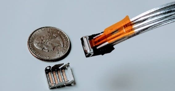
Figure 6 | An example of a cabled transmission line solution: Amphenol’s DensiLink®.
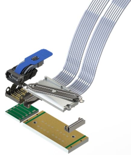
Figure 7 | A second example of a cabled transmission line solution: Amphenol’s micro-LinkOVER™, next to DensiLink®, for relative size comparison.
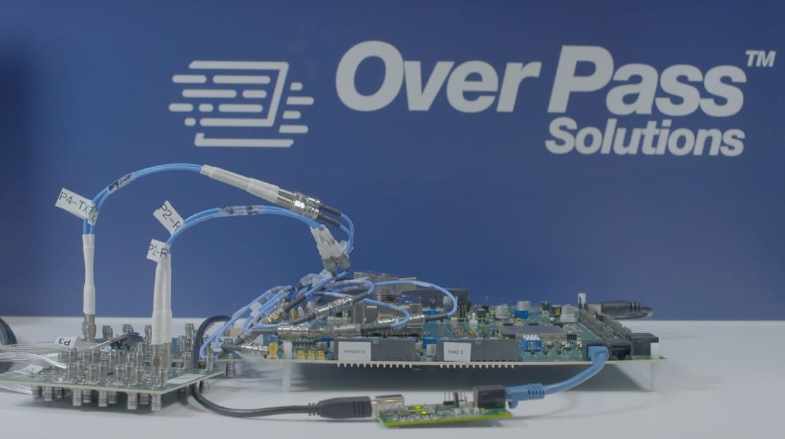
Figure 8 | An OSFP cable assembly working at 112 Gb/s with a cabled transmission line solution and Inphi SerDes.
In summary, cabled transmission line solutions enable integrators to overcome the most difficult signal integrity solutions at 112 Gb/s and beyond by reducing insertion loss with a low reflection technology.
Article contributed by Amphenol Communications Solutions. Visit Amphenol CS to learn more.
Like this article? Check out our other High-Speed articles, our Datacom Market Page, and our 2024 and 2025 Article Archive.
Subscribe to our weekly e-newsletters, follow us on LinkedIn, Twitter, and Facebook, and check out our eBook archives for more applicable, expert-informed connectivity content.